
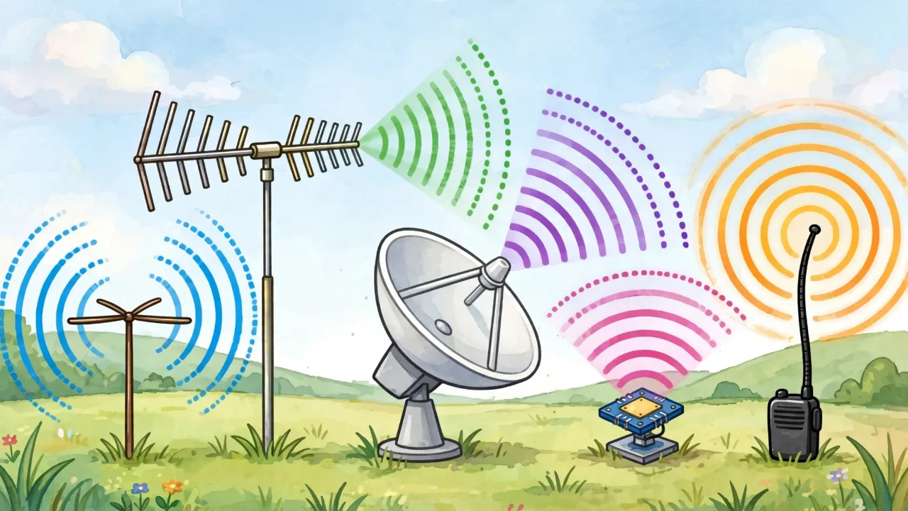
Antennas Catch Invisible Waves 📡

Old TVs had bunny ears on top!

A walkie-talkie has a bendy stick. It catches your friend's voice.

This big bowl looks up at space!

A tiny flat one hides inside your phone. Antennas are everywhere!
Antennas grab invisible waves out of the air. Different shapes catch different waves.
Bunny Ears
Old TVs had two metal rods on top. You moved them until the picture was clear. Each rod is half of a dipole, the simplest antenna of all.
Rubber Duck
Walkie-talkies have a short bendy antenna. It hears in every direction, so you never have to point it.
Dish
The big round dish on a roof catches signals from satellites in space. Its curve bounces every wave to one tiny spot in the middle.
Yagi

This one looks like a fish skeleton. All its rods help it listen in one direction. Rooftop TV antennas are Yagis.
Patch
A tiny flat square hides inside your phone and tablet. WiFi, GPS and Bluetooth all use it.
An antenna turns electricity into radio waves, or catches radio waves and turns them back into electricity. Its shape decides which signals it hears best and which way it listens. Here are nine kinds you can spot.
📏 Dipole

Two straight rods laid end to end, with the cable joined in the middle. It is the simplest antenna, and most others are built from it. For FM radio, a dipole is about as long as a bicycle.
🐰 Bunny Ears

The two rods on an old TV are a dipole you can adjust. They look like rabbit ears, and people moved them around until the picture got clear.
🎯 Yagi

The rooftop antenna with many short bars. Two Japanese inventors, Uda and Yagi, made it in 1926. The extra bars aim the signal one way, like a funnel, so it reaches far.
🏑 Rubber Duck

The short, stubby antenna on a walkie-talkie. A wire is coiled inside a rubber sleeve to keep it small. It works in all directions, so you never have to point it.
🎄 Discone

A flat disc on top of a cone of wires. It can hear a huge range of stations at once, so people who listen to scanners love it.
⭕ Loop

A wire bent into a circle or square. Loops hear almost nothing from one direction, which helps airplanes work out where a signal is coming from.
📡 Dish

The big round dish on a roof collects signals from satellites. Its curve bounces all the waves to one small point, so even a faint signal adds up.
📱 Patch

A flat metal rectangle hidden on a circuit board. It is cheap and tiny, so there is one inside every phone, laptop and GPS.
🌀 Helical

A wire coiled like a spring. Its waves spin as they travel, so a tumbling satellite can still catch them. NASA's early spacecraft used them.
🔧 Try It Yourself
Straighten a wire coat hanger, cut it in half, and tape the halves to a stick with a small gap in the middle. Connect a cable to each half, and you have built a real dipole.
Fun fact: NASA talks to Voyager 1, more than 24 billion kilometers away, with dishes 70 meters wide. By the time the signal arrives, it is billions of times weaker than a watch battery.
Every antenna is a transducer: it converts between guided electromagnetic energy (in a transmission line) and free-space electromagnetic waves. The shape, size, and configuration determine its radiation pattern, bandwidth, impedance, polarization, and gain. Here's how each major type works.
📏 Dipole Antenna
A half-wave dipole is two conductors, each λ/4 long (where λ is the wavelength), fed at the center. The total length equals λ/2. Its radiation pattern looks like a donut: strong broadside, null off the tips. The feed impedance is approximately 73 + j42.5 Ω (about 73 ohms resistive at resonance). Gain is 2.15 dBi. It serves as the reference against which other antennas are measured.
Quick formula: Length (feet) = 468 / frequency (MHz). For a 462 MHz GMRS antenna: 468 / 462 = 1.013 feet, or about 12.2 inches total.
🐰 Bunny Ears / Rabbit Ears
Rabbit ears are a variable-length center-fed dipole. By adjusting the angle and extension of the telescoping elements, users could tune the antenna's resonant frequency and adjust the radiation pattern to favor the direction of the TV transmitter. The V-shape changes the pattern from the donut of a straight dipole to a more complex shape, sometimes providing gain in desired directions. Bunny ears worked for VHF (54-216 MHz), while the attached UHF loop handled 470-806 MHz.
🎯 Yagi-Uda Array

The Yagi uses parasitic elements to create directional gain. The reflector (~5% longer than λ/2) re-radiates energy forward. Each director (~5% shorter) acts as a waveguide, further focusing the beam. Key parameters:
- Gain: ~7 dBi for 3 elements, up to ~17 dBi for 15+ elements
- Front-to-back ratio: 15-25 dB (how much it rejects signals from behind)
- Bandwidth: Narrow, typically 5-10% of center frequency
- Impedance: Adding directors lowers feed impedance; a gamma match or folded dipole driven element compensates
Yagis are used for amateur radio, TV reception, point-to-point links, satellite tracking, and radio astronomy.
🏑 Whip / Rubber Duck
A quarter-wave whip (λ/4 long) works against a ground plane (the radio chassis, a car roof, or the earth). The ground plane mirrors the whip, creating a virtual λ/4 image, so the system behaves like a half-wave dipole. A rubber duck shortens the whip by winding it as a helix, trading efficiency for compactness. A typical rubber duck on a GMRS handheld is about -3 to -6 dBd compared to a full λ/4 whip. Aftermarket antennas like the Nagoya NA-771 recover much of that loss.
🎄 Discone

The discone achieves its wide bandwidth through a smooth impedance transition between the disc and cone elements. The cone length determines the lowest usable frequency (λ/4 at that frequency). Above that, the antenna maintains roughly 50Ω impedance across a 10:1 bandwidth. The radiation pattern is omnidirectional with a slight downward tilt. Gain is modest (0-2 dBi) but the bandwidth is unmatched. Scanner enthusiasts pair discones with wideband receivers to monitor public safety, aviation, marine, and amateur bands simultaneously.
⭕ Loop Antenna
Small loops (circumference < λ/10) act as magnetic antennas, responding to the magnetic field component of EM waves. This makes them less sensitive to local electrical noise. Their figure-8 pattern has two deep nulls perpendicular to the loop plane. Large loops (circumference = λ) have maximum radiation perpendicular to the loop plane and gain of about 3 dBi. The magnetic loop antenna (small tuned loop) is popular for HF amateur radio in restricted spaces because it can be just 1 meter in diameter yet work on 40 meters.
📡 Parabolic Dish

A parabolic reflector focuses parallel incoming rays to a focal point. The gain equation is:
G = η(πDf/c)²
Where D is dish diameter, f is frequency, c is speed of light, and η is aperture efficiency (typically 0.55-0.70). A 3-meter dish at 10 GHz gives about 44 dBi. The beamwidth narrows as gain increases: θ ≈ 70λ/D degrees. Deep Space Network dishes (34-70 meters) achieve gains exceeding 70 dBi, enough to communicate with Voyager 1 at 24 billion km.
📱 Patch / Microstrip Antenna
A patch antenna is a metal rectangle (length ≈ λ/2) on a dielectric substrate above a ground plane. It radiates from the fringing fields at its edges. Single patches provide 5-8 dBi gain with a hemispherical pattern. Bandwidth is narrow (1-5%) unless techniques like stacking or U-slot cutting are used. Phased arrays arrange many patches in grids, controlling the phase of each element to steer the beam electronically without moving parts. This is how 5G massive MIMO, radar, and satellite internet (Starlink) work.
🌀 Helical Antenna
A helical antenna operates in two modes. Normal mode (helix diameter << λ): omnidirectional, similar to a short dipole. Axial mode (helix circumference ≈ λ): produces a focused beam of circular polarization along the helix axis. Axial mode gain is approximately 10-15 dBi depending on the number of turns. Circular polarization eliminates the need for precise alignment between transmitter and receiver, which is why helical antennas are standard for satellite communication, GPS, and radio astronomy.
Antenna theory sits at the intersection of Maxwell's equations, transmission line theory, and signal processing. Every antenna parameter (gain, impedance, radiation pattern, bandwidth, polarization, efficiency) traces back to the boundary conditions of the electromagnetic field at the antenna structure. Here's how each type exploits different physics.
📏 Dipole: The Reference Standard

A center-fed half-wave dipole has an input impedance of 73.1 + j42.5 Ω at exact λ/2 resonance. In practice, shortening it by ~5% brings the reactance to zero, yielding a purely resistive ~68 Ω match. The radiation resistance (73 Ω) represents power radiated as EM waves, while ohmic losses in the conductors are typically negligible for reasonable wire gauges.
The radiation pattern follows E(θ) = cos[(π/2)cosθ] / sinθ, producing a maximum perpendicular to the wire axis. Directivity is 1.64 (2.15 dBi). The dipole defines the dBd scale: 0 dBd = 2.15 dBi.
Variations include the folded dipole (impedance ~292 Ω, 4x standard, useful for matching Yagi feeds), fan dipole (multiple dipoles at different lengths for multiband operation), and cage dipole (thicker effective diameter for wider bandwidth).
🎯 Yagi-Uda: Parasitic Array Theory
The Yagi works through mutual coupling. The driven element induces currents in the parasitic elements. The reflector's current lags (inductive reactance from being longer than resonant), re-radiating energy forward. Directors' currents lead (capacitive reactance from being shorter), acting as a slow-wave structure that guides energy along the array.
Design optimization involves element spacing (typically 0.15-0.25λ), element diameters, and length taper. NEC (Numerical Electromagnetics Code) simulations are standard for Yagi design. The Yagi-Uda gain limit scales roughly as 10*log(N) dBd for N elements, though practical designs plateau around 15-17 dBi due to increasing sidelobes and narrowing bandwidth.
For GMRS base stations, a 5-element Yagi at 462 MHz provides ~10 dBd gain, dramatically extending range in one direction compared to the standard whip.
🏑 Whip / Rubber Duck: Ground Plane Effects

A λ/4 monopole over a perfect ground plane has 36.5 Ω impedance (half the dipole) and 5.15 dBi gain (+3 dB from the ground plane reflection). In practice, ground planes are finite and imperfect. Elevated radials (4 wires at ~45°) approximate an infinite ground plane and raise impedance toward 50 Ω for direct coax connection.
The rubber duck is a normal-mode helical: the helix shortens the physical length while maintaining electrical length. However, the radiation resistance drops dramatically (often below 5 Ω), so most power is dissipated as heat in matching networks. Typical efficiency is 10-30%. A 15 cm rubber duck on a 462 MHz GMRS radio has perhaps -5 dBd effective gain. Upgrading to a full λ/4 whip (16 cm) or λ/2 whip recovers 5-8 dB.
🎄 Discone: Broadband Impedance Theory
The discone is derived from the biconical antenna (two infinite cones tip-to-tip), which has perfectly constant impedance across all frequencies. Replacing one cone with a disc and truncating the other creates a practical broadband antenna. The cone length sets the low-frequency cutoff (where the cone is λ/4). Above that, the impedance remains roughly 50 Ω with VSWR below 1.5:1 across a 10:1 bandwidth.
A discone designed for 25 MHz low cutoff (cone ~3 meters) covers through 250+ MHz, capturing HF, VHF, and UHF in one antenna. This is ideal for SDR (Software Defined Radio) setups monitoring multiple bands with a single receiver like the RTL-SDR.
⭕ Loop: Magnetic Field Coupling

Small loops respond primarily to the magnetic field component (H-field) of the EM wave. The effective aperture is proportional to the loop area squared, so radiation resistance is extremely low: Rr = 31,171(A/λ²)² Ω for a single-turn loop of area A. This makes efficiency a challenge, but a high-Q capacitor-tuned loop concentrates reception in a very narrow bandwidth, rejecting out-of-band interference.
The magnetic loop transmitting antenna is popular in restricted spaces (apartments, HOA-restricted neighborhoods) for HF operation. A 1-meter diameter loop can work 20-10 meters with a remotely tuned vacuum variable capacitor. Bandwidth is only a few kHz, requiring retuning for every frequency change, but the compact size and noise rejection compensate.
📡 Parabolic Dish: Aperture Theory
The parabolic dish is an aperture antenna: its gain is determined by its effective area. The fundamental equation G = 4πAeff/λ² shows gain scales with the square of both diameter and frequency. The f/D ratio (focal length to diameter) determines the feed angle: shallow dishes (f/D = 0.5+) need narrow-beam feeds; deep dishes (f/D = 0.25) need wide-angle feeds.
Key impairments: surface accuracy (RMS errors must be <λ/16 for full gain), blockage (the feed and support struts block some aperture), and spillover (feed radiation that misses the dish). Cassegrain and Gregorian designs use a secondary reflector to relocate the feed behind the dish, reducing blockage and allowing shorter focal lengths.
📱 Patch: Microstrip Theory

The patch antenna can be modeled as a leaky transmission line: the resonant length is λeff/2, where λeff accounts for the dielectric constant (εr) of the substrate. Radiation occurs from the fringing fields at the two radiating edges. The cavity model treats the patch-ground plane gap as a resonant cavity with magnetic current sources at the edges.
Phased arrays are the modern application: hundreds or thousands of patches, each with individual phase shifters and amplifiers. By controlling the relative phases, the beam can be steered electronically in microseconds. This enables massive MIMO (5G), AESA radar (F-35, Patriot missile), and Starlink user terminals (which are flat phased arrays tracking LEO satellites across the sky).
🌀 Helical: Circular Polarization

In axial mode, the helical antenna produces circular polarization because the current travels in a circle. The sense (right-hand or left-hand) depends on the winding direction. Key design parameters: helix circumference C = λ, pitch angle α = 12-15°, number of turns N. Gain ≈ 15*N*(C/λ)²*(S/λ) in linear units, where S is turn spacing.
Circular polarization provides a 3 dB advantage over linear-to-linear in Faraday rotation environments (signals passing through the ionosphere). This is why NOAA weather satellite reception (137 MHz) uses helical or turnstile antennas, and why GPS satellites transmit RHCP (right-hand circular polarization).
📷 Image Credits
Antenna photographs from Wikimedia Commons, used under Creative Commons licenses (CC BY-SA). Yagi: Hustvedt. Discone: KJ4IWX. Parabolic dish: Richard Bartz. Helical: Averse. Rubber duck: CZmarlin. Rabbit ears: WTCA. Loop: M0IDA. Patch: F5ZV. Dipole: Schwarzbeck Mess-Elektronik.
Antenna engineering bridges electromagnetic theory, RF circuit design, and increasingly, computational optimization. This guide covers the nine fundamental antenna topologies with enough depth to select, model, and deploy them for GMRS, amateur radio, scanner, and IoT applications.
📏 Dipole: First Principles
The current distribution on a half-wave dipole approximates a sinusoid: I(z) = I0sin[k(λ/4 - |z|)], peaking at the feedpoint. The far-field pattern in the E-plane follows E(θ) = cos[(π/2)cosθ]/sinθ. Integrating the Poynting vector gives directivity D = 1.643 (2.15 dBi) and radiation resistance Rr = 73.13 Ω.
Practical dipoles deviate from theory due to finite conductor diameter (increasing bandwidth but shifting resonance), proximity to ground (altering pattern and impedance per image theory), and balun requirements (coax is unbalanced; a dipole is balanced). A 1:1 current balun is essential to prevent feedline radiation. For GMRS at 462 MHz, a dipole is 12.2 inches long, easily built from coat hanger wire. Add a PVC cross-boom and you have a base station antenna superior to any stock rubber duck.
🐰 Bunny Ears: Variable Geometry Dipole

The V-dipole (rabbit ears) exploits the relationship between element angle and radiation pattern. At 0° (straight), it is a standard broadside dipole. As the included angle decreases toward 90°, the pattern tilts toward the axis, potentially increasing gain in the forward direction by 1-2 dB. This made bunny ears useful for optimizing reception from a specific transmitter direction without a rotator.
The UHF loop attached to most bunny ear sets is a full-wave loop antenna tuned for the center of the UHF TV band (~600 MHz). Its higher gain (~3 dBi) and broader pattern partially compensated for the higher path loss at UHF frequencies.
🎯 Yagi-Uda: Mutual Impedance Engineering
Yagi design is fundamentally an optimization problem in the mutual impedance matrix. Each element's self-impedance Zii and mutual impedance Zij with every other element determines the current distribution, which in turn defines the radiation pattern. The driven element current is forced by the source; parasitic element currents are induced.
Modern design uses NEC2/NEC4 or FEKO for method-of-moments simulation, with genetic algorithms or particle swarm optimization to find element lengths and spacings that maximize gain, minimize VSWR, and control sidelobe levels. A well-optimized 10-element Yagi achieves 13-14 dBd with 20+ dB F/B ratio and <1.5:1 VSWR across 2% bandwidth.
For GMRS DXing, a 5-7 element Yagi on a mast at 30 feet delivers 10-12 dBd forward gain, equivalent to multiplying your 50W GMRS radio's effective power by 10-16x in the desired direction. Paired with a proper feedline (LMR-400, not RG-58), this setup can achieve reliable simplex contacts at 30-50 miles in favorable terrain.
🏑 Whip / Rubber Duck: Efficiency vs. Convenience
The quarter-wave vertical monopole over a ground plane has theoretical gain of 5.15 dBi (2.15 dBi dipole + 3 dB ground plane). With 4 radials at 45°, feed impedance is approximately 50 Ω. The ground plane can be elevated (radials in free space) or surface-mounted (ground rods, buried radials). NEC models show diminishing returns beyond 16 radials for elevated installations.
The rubber duck compromise: a helically wound monopole with physical length 1/10 to 1/4 of λ/4. Radiation resistance drops to 1-10 Ω, while the matching network introduces losses. Combined efficiency: 10-30%. The aftermarket antenna market thrives on this: a Nagoya NA-771 ($10) on a Baofeng/GMRS HT adds 5-8 dB effective gain over the stock rubber duck. For serious work, a λ/2 J-pole or slim jim (no ground plane required, ~4 dBd) is the gold standard for handheld and base station use.
🎄 Discone: The Scanner Antenna
The discone's broadband behavior derives from its approximation of the infinite biconical antenna, whose impedance is frequency-independent: Z = 120*ln(cot(θ/2)) Ω, where θ is the cone half-angle. A disc-cone half-angle of about 30° yields ~50 Ω. The truncated cone introduces a low-frequency cutoff where cone length = λ/4.
For scanner/SDR applications, the Diamond D-130NJ (25-1300 MHz) or homebrew equivalents are standard. Pair with an RTL-SDR or Airspy for monitoring public safety (MPKA 488 MHz), aircraft (108-137 MHz AM, 978/1090 MHz ADS-B), marine (156 MHz), GMRS (462 MHz), amateur (144/440 MHz), and cellular (700-2100 MHz) simultaneously. The discone is receive-only for most practical purposes; its gain is too low and pattern too broad for effective transmission.
⭕ Loop: Magnetic Coupling and Noise Rejection
The small transmitting loop (STL) has gained popularity for HF operation in restricted environments. The radiation resistance Rr = 31,171(A/λ²)² Ω means a 1m diameter loop on 20m (14 MHz) has Rr ≈ 0.003 Ω. Efficiency depends entirely on minimizing ohmic loss: copper or aluminum tube (not wire), soldered/welded joints, and a high-Q vacuum variable capacitor (Q > 5000). Total Q of 500-1000 is achievable, yielding 50-80% efficiency on 20-10 meters but dropping to 10-20% on 40m.
The deep nulls perpendicular to the loop plane provide 20-30 dB of noise rejection when oriented to null interference sources. This noise advantage often compensates for the gain deficit versus a dipole, particularly in urban/suburban environments with high ambient noise floors.
For direction finding, the Adcock array (four vertical dipoles in a square) avoids the polarization errors of simple loops at HF frequencies.
📡 Parabolic Dish: Aperture Efficiency and Feed Design
The gain equation G = η(4πA/λ²) = η(πDf/c)² encapsulates the physics. Aperture efficiency η accounts for illumination taper, spillover, blockage, surface errors, and feed mismatch. Typical η = 0.55-0.70 for prime-focus feeds; Cassegrain designs achieve 0.65-0.75.
The Ruze equation quantifies surface accuracy requirements: gain loss = exp(-(4πσ/λ)²), where σ is RMS surface error. For less than 1 dB loss, σ < λ/16. At 10 GHz (λ = 30mm), surface accuracy must be <1.9 mm.
For amateur Earth-Moon-Earth (EME) communication at 1296 MHz, enthusiasts use 3-5 meter dishes with ~35 dBi gain. The Deep Space Network's 70m dishes at Goldstone achieve 74 dBi at X-band, communicating with Voyager 1 at 23.5 billion km using 23W of transmit power from the spacecraft.
📱 Patch: Phased Array and Beamforming
The rectangular patch resonates when length L ≈ λeff/2 = c/(2f√εr,eff). The effective dielectric constant εr,eff accounts for fringing: εr,eff ≈ (εr+1)/2 + (εr-1)/2 * (1+12h/W)-1/2, where h is substrate height and W is patch width.
Modern phased array systems are defined by the array factor AF = Σanexp(jn(kd*sinθ + β)), where an is element amplitude, d is element spacing, and β is the progressive phase shift. Beam steering is accomplished by varying β. Element spacing d ≤ λ/2 prevents grating lobes.
Starlink user terminals contain 1,280 dual-polarized patch elements on a flat panel, electronically tracking LEO satellites from horizon to horizon. 5G massive MIMO panels use 64-256 elements with digital beamforming to simultaneously serve dozens of users with individual beams. This is arguably the most consequential antenna technology of the 2020s.
🌀 Helical: Axial Mode Design
Axial-mode design parameters: circumference C = λ, pitch angle α = 12-14°, turn spacing S = C*tan(α) ≈ λ/4, ground plane diameter ≥ 3λ/4. The number of turns N determines gain: G ≈ 15*N*C²*S/λ³ (linear). For 10 turns: ~14 dBi RHCP.
The axial ratio (AR) measures circular polarization purity: AR = 1.0 is perfect CP, AR = ∞ is linear. Well-designed helicals achieve AR < 2 dB over a 1.7:1 bandwidth. The quadrifilar helix (QFH) is a variant with four interleaved helices, producing a cardioid pattern ideal for NOAA APT satellite reception at 137 MHz. A QFH built from coax cable and PVC pipe is a classic amateur radio project.
For amateur satellite work, a pair of crossed Yagis (one horizontal, one vertical, fed 90° apart) achieves circular polarization with higher gain than a helical, but requires more mechanical complexity and a phasing harness.
🔧 Choosing the Right Antenna
The selection matrix for practical applications:
- GMRS base station: 5-element Yagi (directional) or J-pole/collinear (omnidirectional), fed with LMR-400
- GMRS handheld: Replace the rubber duck with a Nagoya NA-771 or Signal Stick
- Scanner/SDR monitoring: Discone (wideband) or dedicated Yagi (single band, higher gain)
- HF amateur, restricted space: Magnetic loop or end-fed half-wave with a 49:1 unun
- Satellite reception (NOAA/ISS): QFH or crossed Yagis with elevation rotator
- WiFi/Bluetooth extension: Patch array or cantenna (waveguide)
- Direction finding: Small loop with null steering, or phased Adcock array
The single most impactful upgrade for any radio system is almost always the antenna. A $10 antenna upgrade typically outperforms a $100 amplifier upgrade, because the antenna improves both transmit and receive while adding no noise.
📷 Image Credits
Antenna photographs from Wikimedia Commons, Creative Commons licensed. Yagi: Hustvedt CC BY-SA 3.0. Discone: KJ4IWX CC BY-SA 3.0. Parabolic dish: Richard Bartz CC BY-SA 2.5. Helical: Averse CC BY-SA 3.0. Rubber duck: CZmarlin CC BY-SA 4.0. Rabbit ears: WTCA CC BY-SA 3.0. Loop: M0IDA CC BY-SA 4.0. Patch: F5ZV CC BY-SA 3.0. Dipole: Schwarzbeck CC BY-SA 3.0.